SLAM

Collaborators: \

This project is to implement a simple mapping and localization algorithm in an indoor environment. TO do so, we employ a particle filter which uses information from an IMU and a LiDAR sensor. Specifically, the particle filter is used to localize the agent and the best particle (instead of all particles in general cases) is used to update the map.

Localization

Let’s start with the partical filter.

Particle filters (PFs) are a generalization of Unscented Kalman Filters that can handle non-Gaussian filtering distributions. Specifically, a PF utilizes the notion of importance sampling to estimate the distribution of robot’s state. The positions (values) \(x^{(i)}\) together with the weights \(w^{(i)}\) of the particles decribe the estimation of the target distribution as a sum of Dirac-delta distributions at points \(x^{(i)}\), as shown in the figure below.

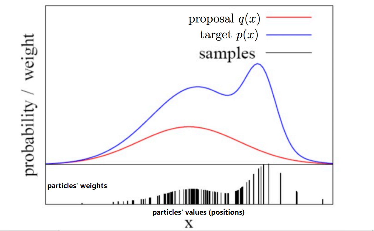
The key questions are

• How do we sample the values of particles?
• How do we update the weights of the particles?

in order to best approximate the actual distribution of the robot’s state.

For the first question, the values of the particles are first changed by propagating the dynamics and then changed by the resampling process. For the second question, the weight of each particle is scaled propotionally to the likelihood of receiving current observation and then the sum of the weights are normalized to one. In addition, the resampling process will make all weights equal while keeping the estimated distribution unchanged. Here is the algorithm

1. Propagating the dynamics

   for each particle i = 1, . . . , n, update particles by one timestep

   \(x^{(i)}_{k+1 \mid k} = f(x^{(i)}_{k \mid k}, u_k) + \epsilon_k\), where \(f\) is the system dynamics, \(\epsilon_k \sim \mathcal{N} (0, \mathbf{R})\) is Gaussian noise. Weights of particles are unchanged \(w^{(i)}_{k+1\mid k} = w^{(i)}_{k\mid k} = 1/n\).

2. Incorporating the observation

   for each particle i = 1, . . . , n, scale the weight using the likelihood of receiving that observation

   \(w^{(i)}_{k+1\mid k+1} \propto P(y_{k+1} \mid x^{(i)}_{k+1 \mid k}) w^{(i)}_{k+1\mid k}\)

   In this project, \(P(y_{k+1} \mid x^{(i)}_{k+1 \mid k})\) is given by \(e^{\sum_{ij \in O}m_{ij}}\), where \(O\) is the set of occupied cells as detected by the LiDAR scan assuming the robot is at particle \(p\) and \(m_{ij}\) is our current estimate of the binarized map.

3. Normalizing the weights

   the weights \(w^{(i)}_{k+1\mid k+1}\) to sum up to 1.

4. Resampling step

   Perform the resampling step to obtain new particle locations \(x^{(i)}_{k+1 \mid k+1}\) with uniform weights

Resampling step

The resampling step takes particles \({w^{(i)}, x^{(i)}}^n_{i=1}\) which approximate a probability density \(p(x)\)

and returns a new set of particles \(x'^{(i)}\) with equal weights \(w'^{(i)} = \frac{1}{n}\) that approximate the same probability density

The goal of the resampling step is to avoid particle degeneracy, i.e., remove unlikely particles with very low weights and effectively split the particles with very large weights into multiple particles.

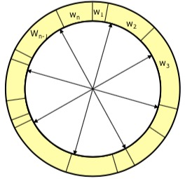
Consider the weights of particles \(w^{(i)}\) arranged in a roulette wheel as shown above. We perform the following procedure: we equally divide the wheel into n areas. We randomly pick a location at each area and add the corresponding particle into our set \({x'^{(i)}}\) Since particles with higher weights take up a larger angle in the circle, this procedure will often pick those particles and quickly move across particles with small weights without picking them too often. As an algorithm

• initialize \(i = 1\), \(c = w^{(1)}\) and let \(r\sim Uniform(0,\frac{1}{n})\)
• For each \(m = 1, . . . , n\), let \(u = r+(m-1)/n\). Increment \(i \leftarrow i+1\) and \(c \leftarrow c +w^{(i)}\) while \(u > c\) and set new particle location \(x'^{(m)} = x^{(i)}\).

Update Map

Using the particle with largest weight, we increase a map_t.log_odds array at cells that are recorded as obstacles by the LiDAR by slam_t.log_odds_occ and decrease the values in all other cells inside the LiDAR’s vision by log_odds_free. We also clip the map_t.log_odds to lie between [-slam_t.map.log_odds_max, slam_t.map.log_odds_max] to prevent increasingly large values in the log_odds array. The cells with corresponding log_odds larger than a threshold will be treated as occupied, otherwise will be treated as free cells.

Code and Implementation

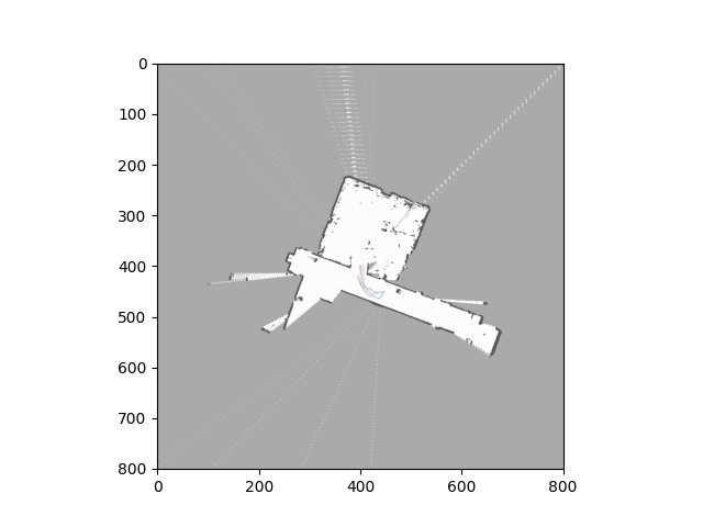
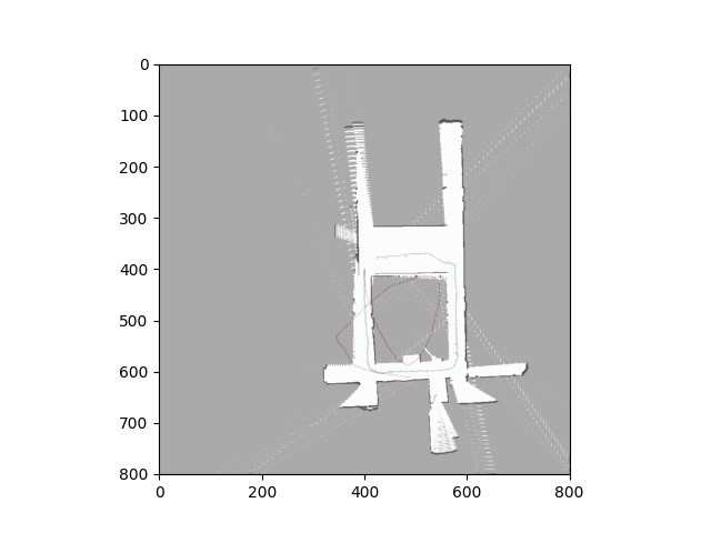
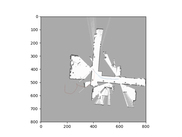
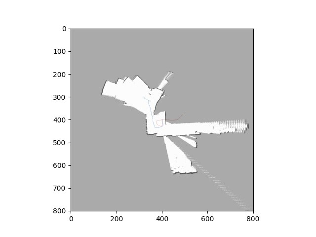
We test the SLAM algorithm with the data collected from a humanoid named THOR in indoor environment. The implementation datails, which involve some 3D transformation since the robot has a 2-DoF neck, are omitted here. The code can be found HERE. Just downloading it and running main.py should work!

Preliminary Results